Better late than never

CESS Researcher Roberto Cerina and Director Raymond Duch partnered with UCL Statistics Professor Gianluca Baio to test a novel methodology to estimate constituency-level results from publicly available individual level datasets and publicly available opinion polls. To this end, they produced estimates of vote shares and headline seats for the 2019 UK General Election. The results of this efforts, as well as basic details of the methodology, follow. This post was published before the election returns on http://www.statistica.it/gianluca/post/2019-12-12-better-late-than-never/.

Summary

It should be noted the methodology and results presented below are highly experimental and derived from significant simplification and approximation to meet the impending election date. We plan to continue working on these ideas to improve them. Thus, the methods will likely undergo significant modification before being presented at conferences and published as a paper. Nonetheless, we thought the results were interesting enough to share with the wider public. We predict the conservatives will lead labour by around 6 percentage points, which will translate to 27 seats over the threshold for an absolute majority in parliament for a total of 353 seats, with a 95% prediction interval of seats ranging from -1 (hence a hung parliament) to 55.

Method

We propose a novel methodology to produce dynamic election forecasts using exclusively publicly available data. The ethos of this work builds on two literatures: i) the literature on Multilevel Regression and Post-Stratification (MRP) and its general form of Regularized Regression and Post-Stratification (RRP); ii) the literature on pooling the polls and modeling campaign dynamics.

In short, the methodology takes full advantage of a Bayesian approach in combining different sources of evidence; firstly we consider a large survey (e.g. the British Election Study), which we use to estimate structured (“random”) effects of interest from the individual level data. In particular, we focus especially on constituency-level deviations from the global average voting share of each party. We then update the global mean using the latest public opinion polls. In particular, we consider the data published by pollsters in the form of univariate cross-tabulations (e.g. voting intention by age group; or voting intention by sex; ect). Finally, we produce voter-category-level estimates using the updated global mean and the constituency-level effects estimated in the first step, and post-stratify these to a stratification frame to obtain constituency-level results.

The Constituency-level estimates of the vote for each party are then tallied up and a winner is declared in each; in principle this procedure can easily provide credible uncertainty estimates by merging individual-level and polls-level uncertainty – note that this step is omitted in this brief exposition.

Data

The procedure requires three data sources:

1. a recent (and relevant) publicly available source of individual-level voting intention, and associated individual- and constituency-level characteristics. In the UK, one relevant example is represented by the British Election Study (BES), and in particular wave 16 of the Online Panel was most relevant to the election at hand. The advantage of using the BES is that it is publicly available and has a relatively large sample size, with a wealth of covariates investigated. However, it is possible to include large specific surveys (possibly privately owned, but accessible to the researchers);
   
2. A daily tally of published opinion polls, at the cross-tab level (i.e. voting intention by age groups or Brexit vote), conditional on turnout;
   
3. The latest census data and any further information to model a stratification-frame (a vector of voter-categories and associated size within the electorate) on which to stratify our individual-level estimates.

Step 3. is a separate modeling exercise, which deserves a degree of attention we cannot devolve in this short piece, and so the reader should just assume it as given for now.

Modelling

Obtaining reasonable priors and constituency-level information from the British Election Study (BES)

We model the vote-choice for parties $j=1\dots <!--\; \dots \; -->,J$ assuming they are categorically distributed (multinomial with $N=1$) for each individual in the BES sample $$v_{ij}\sim <!--\; \sim \; -->\text{Categorical}({\mathit{\pi <!--\; \pi \; -->}}_i),$$

Where ${\mathit{\pi <!--\; \pi \; -->}}_i={\mathrm{\pi <!--\; \pi \; -->}}_{i1},\dots <!--\; \dots \; -->,{\mathrm{\pi <!--\; \pi \; -->}}_{iJ}$ is a vector of individual-level and party specific probabilities.

We model (on the logit scale) the mean probability μ_ij of voting for any of the parties at hand on the logit scale:

$${\displaystyle {\pi }_{ij}=\frac{\exp \left({\mu }_{ij}\right)}{\sum _{j=1}^J\exp \left({\mu }_{ij}\right)};}$$

the model involves a party-level intercept ${\mathrm{\alpha <!--\; \alpha \; -->}}_j$ a series of random effects ${\mathrm{\beta <!--\; \beta \; -->}}_{jko[k]}$ where each $k=1,\dots <!--\; \dots \; -->,K$ represents an individual-level characteristic of the voter, such as “Age”, “Past Vote” or “Parliamentary Constituency”, and the index $o=1,..,O[k]$ indicates the level of the given characteristic – say k indicates “Age”, and we have age categories “18 to 34”, “35 to 54”, “55 to 64”, “65 plus”, represented by $o=1,\dots <!--\; \dots \; -->,4$ The final piece of the model is an area-level predictor $Z$ involving $a=1,\dots <!--\; \dots \; -->,A$ variables at the constituency-level, such as “%Leave”, “%Level4 Education” and others. The area-level predictor is needed to soften the MRP tendency to produce attenuation bias, by selectively relaxing the level of shrinkage on the constituency effects. These assumptions imply a model for ${\mathrm{\mu <!--\; \mu \; -->}}_{ij}$ as the following

$${\mathrm{\mu <!--\; \mu \; -->}}_{ij}={\mathrm{\alpha <!--\; \alpha \; -->}}_j+\underset{k=1}{\overset{K}{\sum <!--\; \sum \; -->}}\underset{o=1}{\overset{O[k]}{\sum <!--\; \sum \; -->}}{\mathrm{\beta <!--\; \beta \; -->}}_{jko[k]}+\underset{a=1}{\overset{A}{\sum <!--\; \sum \; -->}}{\mathrm{\theta <!--\; \theta \; -->}}_{ja}{Z}_{ia}.$$

The following priors are assigned to the model parameters: no shrinkage is sought in the party-intercepts, which are assigned non-informative, independent normal priors; the area-predictor is assigned a ridge-prior to encourage stability where party-specific sample sizes are very small (as is the case for Plaid Cymru for instance); the random effects are given non-informative priors with a shared variance component, in order to encourage shrinkage and avoid over-fitting. The variance components are given (mostly) non-informative conjugate priors to encourage fast convergence given the size of the dataset and stringent time requirements (but of course, we will explore more structured alternatives soon).

$$\begin{array}{rcl}{\mathrm{\alpha <!--\; \alpha \; -->}}_j& \sim <!--\; \sim \; -->& \text{Normal}(0,{\mathrm{\psi <!--\; \psi \; -->}}_j)\\ {\mathrm{\beta <!--\; \beta \; -->}}_{jko[k]}& \sim <!--\; \sim \; -->& \text{Normal}(0,{\mathrm{\tau <!--\; \tau \; -->}}_k)\\ {\mathrm{\theta <!--\; \theta \; -->}}_{ja}& \sim <!--\; \sim \; -->& \text{Normal}(0,{\mathrm{\tau <!--\; \tau \; -->}}_{\mathrm{\theta <!--\; \theta \; -->}})\\ {\mathrm{\psi <!--\; \psi \; -->}}_j,{\mathrm{\tau <!--\; \tau \; -->}}_k,{\mathrm{\tau <!--\; \tau \; -->}}_{\mathrm{\theta <!--\; \theta \; -->}}& \stackrel{iid}{\sim <!--\; \sim \; -->}& \text{Gamma}(\mathrm{ϵ<!--\; ϵ\; -->},\mathrm{ϵ<!--\; ϵ\; -->}).\end{array}$$

Care is taken to ensure the model is fully identifiable, implementing a corner-constraint such that all coefficients for $j=$ “Conservatives” are set to zero.

Modeling cross-tabs from publicly available Opinion Polls

All the effects estimated from the previous model, with the exception of the constituency level random effects and area level predictors (save these aside for now), are used as informative priors in the model of opinion polls.

We do not limit ourselves to analyzing the headline shares published daily, but have built a dataset of published cross-tabs for the most important breakdowns, such as age-groups, education level, gender, past vote etc.; note there is no breakdown published by pollsters at the constituency-level¹ and hence we cannot update the constituency-level effects estimated in the first phase. We only look at breakdowns conditional of likely voters.

For each characteristic $o[k]$ (i.e. “Age Group – 18 to 24”), on a given day-to-election $t=T,\dots <!--\; \dots \; -->,0$ a polling house $h=1,\dots <!--\; \dots \; -->,H$ will publish a vote-breakdown by party $j$; we can model these counts according to a multinomial distribution as follows:

$$V_{o[k]hjt}\sim <!--\; \sim \; -->\text{Categorical}(p_{o[k]h1t},\dots <!--\; \dots \; -->,p_{o[k]hJt});$$

once again we implement a logit-link:

$${\displaystyle p_{o[k]hjt}=\frac{\exp <!--\; \; -->\left({\mathrm{\eta <!--\; \eta \; -->}}_{o[k]hjt}\right)}{\underset{j=1}{\overset{J}{\sum <!--\; \sum \; -->}}\exp <!--\; \; -->\left({\mathrm{\eta <!--\; \eta \; -->}}_{o[k]hjt}\right)};}$$

the model involves the familiar individual-level parameters as before, with a couple of differences: i) the party-intercepts now move over-time to the tune of a random walk, allowing for exponential discounting of past observations and dynamic estimation of the national campaign effect; ii) given the change in nature of the observations, which are now aggregated counts at the characteristic level, we estimate each characteristic effect ${\mathrm{\beta <!--\; \beta \; -->}}_{jo[k]}$ separately, but ensure they have the same random-effect structure across equations; iii) parameter ${\mathrm{\delta <!--\; \delta \; -->}}_{jo[k]h}$ is introduced, which seeks to identify and remove the “house effect” at the characteristic level – i.e. how much higher/lower does, say, YouGov estimate the $j-<!--\; -\; -->$ vote amongst 18 to 24 year olds, compared to the average pollster?

The linear predictor is defined as

$${\mathrm{\eta <!--\; \eta \; -->}}_{o[k]hjt}={\mathrm{\alpha <!--\; \alpha \; -->}}_j+{\mathrm{\beta <!--\; \beta \; -->}}_{jko[k]}+{\mathrm{\delta <!--\; \delta \; -->}}_{jo[k]h}.$$

Note that again care is taken to impose identification constraints: the same corner-constraint on the conservative coefficients is imposed, as well as a sum-to-zero constraint over houses to identify the bias parameter.

The priors follow; note that the ${}^{\ast <!--\; \ast \; -->}$ sign indicates that the parameter value is set to point estimate from the individual-level model, so that the posterior will be an average of the polls and BES prior.

$$\begin{array}{rcl}{\mathrm{\alpha <!--\; \alpha \; -->}}_{jt}& \sim <!--\; \sim \; -->& \text{Normal}({\mathrm{\alpha <!--\; \alpha \; -->}}_{jt+1},{\mathrm{\tau <!--\; \tau \; -->}}_{\mathrm{\alpha <!--\; \alpha \; -->}})\\ {\mathrm{\alpha <!--\; \alpha \; -->}}_{jT}& \sim <!--\; \sim \; -->& \text{Normal}({\mathrm{\alpha <!--\; \alpha \; -->}}_j^{\ast <!--\; \ast \; -->},{\mathrm{\psi <!--\; \psi \; -->}}_j)\\ {\mathrm{\beta <!--\; \beta \; -->}}_{jko[k]}& \sim <!--\; \sim \; -->& \text{Normal}({\mathrm{\beta <!--\; \beta \; -->}}_{jko[k]}^{\ast <!--\; \ast \; -->},{\mathrm{\tau <!--\; \tau \; -->}}_{\mathrm{\beta <!--\; \beta \; -->}o[k]}^{\ast <!--\; \ast \; -->})\\ {\mathrm{\delta <!--\; \delta \; -->}}_{jo[k]h}& \sim <!--\; \sim \; -->& \text{Normal}(0,{\mathrm{\tau <!--\; \tau \; -->}}_{\mathrm{\delta <!--\; \delta \; -->}})\\ {\mathrm{\tau <!--\; \tau \; -->}}_{\mathrm{\gamma <!--\; \gamma \; -->}}& \sim <!--\; \sim \; -->& \text{Gamma}(0.01,1)\end{array}$$

Obtaining local predictions and stratifying

The last step of our effort involves producing group-level predictions to stratify. We identify groups $g=1,\dots <!--\; \dots \; -->,G$ as the mutually exclusive combination of all voter-characteristics described above – so for instance $g=1$ can stand for the category “Age: 18 to 24; Vote2017: Labour; BrexitVote: Remain; Education: Level4”. For each of these groups we produce a vote-probability distribution ${\mathrm{\varphi <!--\; \varphi \; -->}}_{jga}$ based on the predictions from the updated model. For each constituency $a=1,\dots <!--\; \dots \; -->,A$ we seek to aggregate over the groups according to their population weights conditional on turnout, $N_{ga}$ and obtain constituency estimates of vote share ${\mathrm{\rho <!--\; \rho \; -->}}_{ja}$

$$\begin{array}{rcl}{\mathrm{\varphi <!--\; \varphi \; -->}}_{jga}& =& {\stackrel{^<!--\; ^\; -->}{\mathrm{\alpha <!--\; \alpha \; -->}}}_{j0}+\underset{k=1}{\overset{K}{\sum <!--\; \sum \; -->}}\underset{o=1}{\overset{O[k]}{\sum <!--\; \sum \; -->}}{\stackrel{^<!--\; ^\; -->}{\mathrm{\beta <!--\; \beta \; -->}}}_{jko[k]}+{\stackrel{^<!--\; ^\; -->}{\mathrm{\theta <!--\; \theta \; -->}}}_{ja}{Z}_{ia}\\ {\displaystyle {\mathrm{\Phi <!--\; \Phi \; -->}}_{jga}}& =& \frac{\exp <!--\; \; -->\left({\mathrm{\varphi <!--\; \varphi \; -->}}_{jga}\right)}{\underset{j=1}{\overset{J}{\sum <!--\; \sum \; -->}}\exp <!--\; \; -->\left({\mathrm{\varphi <!--\; \varphi \; -->}}_{jga}\right)}\\ {\displaystyle {\mathrm{\rho <!--\; \rho \; -->}}_{ja}}& =& \frac{\underset{g=1}{\overset{G}{\sum <!--\; \sum \; -->}}{\mathrm{\Phi <!--\; \Phi \; -->}}_{jga}{N}_{ga}}{\underset{g=1}{\overset{G}{\sum <!--\; \sum \; -->}}{N}_{ga}}.\end{array}$$

Some results

So: the model produces a wealth of possible outcomes. For example, we can estimate the overall vote share from the “deep-polls” cross-tabulations, accounting for the underlying correlation in the several univariate cross-tabs. The model predicts the following overall vote share (rounded up).

Party	Vote share
Conservative	43%
Labour	37%
Liberal Democrats	12%
SNP/PC	4%
Green	2%
Brexit Party	1%
Other	1%

We can then translate these into constituency level values, to determine the composition of the next parliament. Based on the outcome of the (again: relatively preliminary version of the) model, the Tories should be 27 seats over the threshold for an absolute majority in parliament for a total of 353 seats; a healthy margin of error should be placed on these; following the same standard deviation of the YouGov MRP projections, the 95% prediction interval for this call is [-1,55]. Hence our model includes the possibility of a hung parliament, albeit with very low probability.

We can also explore the “house” effect (ie the impact of different pollsters on the several cross-tabulated covariates). Something like in the following graph.

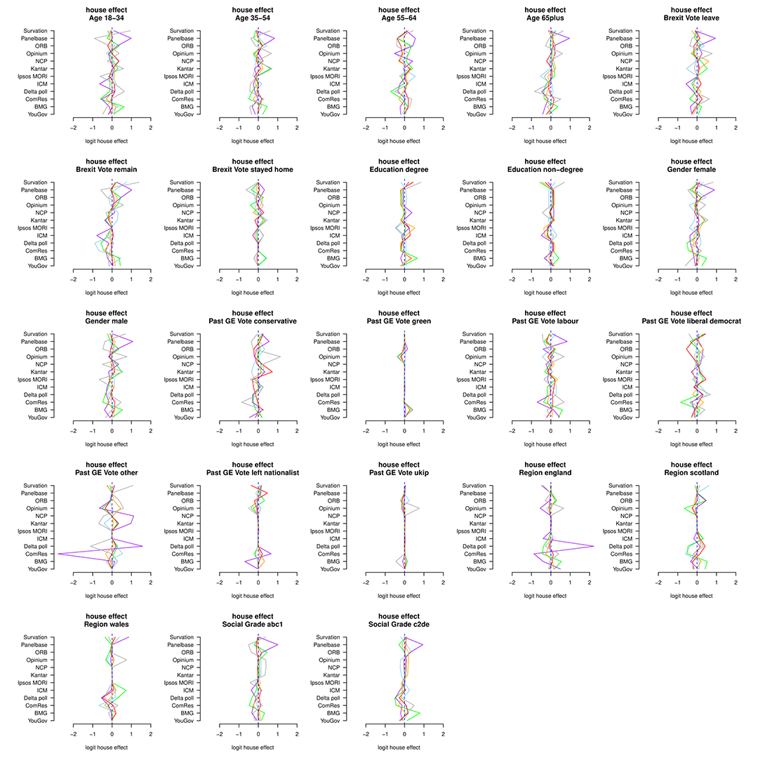
The plots show the house-bias (relative to the average house’s pro-conservative bias) for each party, for each voter-characteristic (the color scheme is the same as for the campaign dynamic plot below). The idea here is that big swings (say 2 standard deviations away from 0) to the left or the right of the conservative baseline should identify house effects which are out of the ordinary and prompt further scrutiny of the pollster. Note that the conservative baseline makes the interpretation less intuitive, but it is a necessary evil to identify the model.

Or, we could explore the campaign dynamics — for instance, relatively to the baseline (eg the Conservatives, in this case)

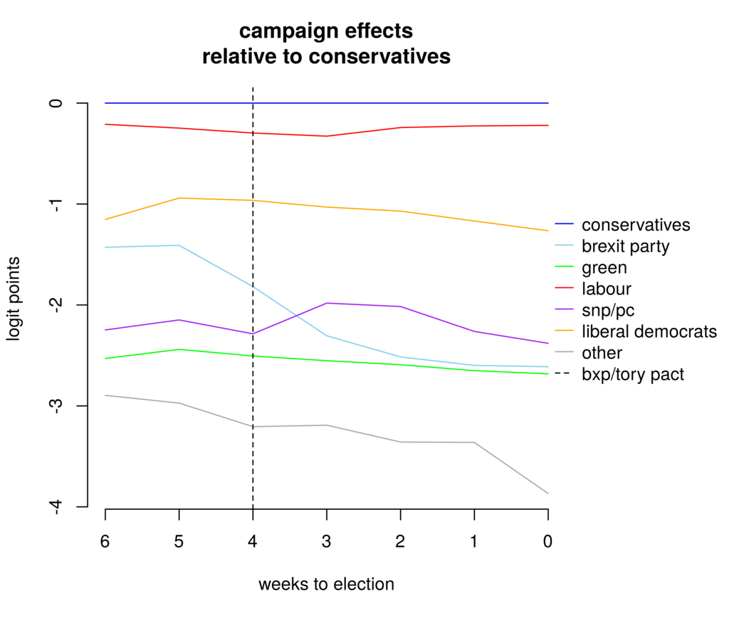
which shows how Labour was slowly, slowly catching up.

Of course, we can compute all relevant posterior probabilities (eg actually probability of a given majority, hung parliament, geographical distributions, etc). For now, we’re not reporting on all the details — but we’ll keep working on the model and use the actual results that will be revealed later and tomorrow, to validate and improve on it.

Conclusions

So, in summary, the main idea is to use Bayesian hierarchical modelling to essentially bring some correlation in the many univariate cross-tabulations that are publicly available from the various pollsters. More care needs to be taken to fine-tune predictions at the constituency level, but for now our model creates a much finer estimate from just the polls, which can be complemented with large surveys or historical trends (eg local constituency to overall, or region). The overall aim of this project is to make MRP-like areal estimation available to researchers without the resources to collect hundreds of thousands of individual respondents.

---

1. If MRP estimates (e.g. from Yougov and others) were available, we could eventually incorporate those in, though it should be noted that they are of quite different in nature to traditional polling, and would require ad-hoc model specification. ↩